Mixer Image Rejection: Image Frequency and LO Side Selection

Mixer image rejection starts with the image frequency formula: f_image = 2f_LO − f_RF. For a conventional receiver with a nonzero difference IF and two positive RF sidebands, high-side LO injection places the image above the wanted RF; low-side injection places it below. The wanted signal and its image are separated by twice the IF. Select the LO side by comparing the resulting image bands, then allocate rejection between RF preselection and the complete image-reject mixer path.

An ordinary IF filter cannot separate two signals already converted to the same frequency in a single real IF output. The useful calculation is therefore how much image energy reaches that output after RF filtering and any I/Q cancellation. This guide is part of the RF signal-chain collection; use RF, IF and LO explained for the underlying frequency roles.

Frequency-plan input	Symbol and units	What to establish
Wanted RF	f_RF, MHz or GHz	Center frequency and occupied band edges
Intermediate frequency	f_IF, same units as RF	Positive difference frequency at the selected output
Local oscillator	f_LO, same units as RF	High-side or low-side choice, available tuning range and required drive
Image band	f_image, same units as RF	Reflection of the wanted band about the fixed LO
Desired-to-image margin	M, dB	Required output ratio under the project’s blocker conditions

Calculate the image: high-side vs. low-side LO injection

Solve both injection choices before selecting a preselector. With f_IF = |f_RF − f_LO|, the two RF frequencies that produce the same real IF are f_LO − f_IF and f_LO + f_IF. Their sum is twice the LO, giving f_image = 2f_LO − f_RF. MITEQ’s Image Rejection Mixers/QIFMs, Q1, describes this mirror relationship and identifies interference, spurs and spectrum inversion as LO-selection considerations.

Relationship	High-side LO	Low-side LO
LO relative to wanted RF	Above	Below
LO calculation	f_LO = f_RF + f_IF	f_LO = f_RF − f_IF
Image calculation	f_image = f_RF + 2f_IF	f_image = f_RF − 2f_IF
Image position	Above wanted RF and LO	Below wanted RF and LO
Wanted-to-image spacing	2f_IF	2f_IF
Spectral order at fixed LO	Reversed at the real difference IF	Preserved at the real difference IF

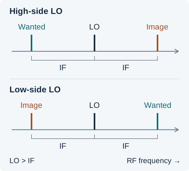
The two-positive-sideband model requires f_LO > f_IF. For the low-side row, that means f_RF > 2f_IF. If the lower image calculation is zero or negative, analyze the actual sum/difference conversion plan instead of taking its absolute value and retaining the same spacing rule. Zero-IF and harmonic mixing require their own frequency analysis.

Spectral inversion follows directly from the fixed-LO equations. With high-side injection, increasing RF decreases f_LO − f_RF; with low-side injection, increasing RF increases f_RF − f_LO. Check that the demodulation or subsequent frequency conversion expects the resulting orientation. Neither injection side inherently supplies more rejection: its advantage comes from where the image lands relative to interferers and the filter response.

Worked frequency example: a published calibration configuration

Analog Devices’ AN-1258, Image Rejection Calibration on the ADF7021, ADF7021-N, and ADF7021-V, uses a 100 kHz IF and an internal image-calibration tone at 870.84 MHz, with the receiver programmed to 871.04 MHz. Applying the low-side equations to that configuration:

With f_IF = 0.10 MHz, the calculated LO is 871.04 − 0.10 = 870.94 MHz, and the image is 2 × 870.94 − 871.04 = 870.84 MHz. The wanted RF and image sit 100 kHz on either side of the LO, giving 200 kHz wanted-to-image separation.

For a finite wanted band, calculate both image edges at each LO setting. At fixed LO, a wanted band from f_low to f_high maps to the image interval 2f_LO − f_high through 2f_LO − f_low. Test filter rejection across that interval; a center-frequency marker can miss its weakest edge.

Convert the image blocker into a preselector requirement

Budget differential attenuation: image-band filter loss minus wanted-band filter loss. A filter attenuating the image also reduces the wanted signal by its passband insertion loss. Only the difference improves the desired-to-image ratio. The Mini-Circuits technical note IQ Mixers: Image Reject Down-Conversion & Single Sideband Up-Conversion, under “Mixer Basics,” explains why low IF makes this filtering harder: the wanted RF and image move closer together.

Use one common receiver input reference plane for the desired and image powers:

Variable	Definition	Unit
P_D, P_I	Desired input power and worst image-band interferer power	dBm
L_D, L_I	Positive preselector insertion loss at desired RF and image RF	dB
A_pre = L_I − L_D	Differential preselector rejection	dB
R_mix = G_D − G_I	Desired-minus-image conversion gain of the complete mixer/combiner path, measured with equal RF input powers	dB
M	Required output desired-to-image margin	dB

In a linear path, the two output powers are:

• Desired: P_D,out = P_D − L_D + G_D.
• Image: P_I,out = P_I − L_I + G_I.

Subtracting them gives the output margin and the rejection requirement:

D/I_out = P_D − P_I + A_pre + R_mix

A_pre + R_mix ≥ P_I − P_D + M

Thus the remaining mixer requirement is R_mix ≥ P_I − P_D + M − A_pre, before adding the project’s uncertainty and design allowance. If a negative residual results, the filter already meets this ratio requirement; noise, spurs and overload still need their own checks.

Use the weakest differential attenuation over the relevant bands and operating conditions. Include any intervening LNA’s frequency-dependent gain explicitly, once, rather than hiding it in both preselector and mixer rejection. Keep the input reference plane and the boundary of each gain term fixed when comparing architectures.

If the filter plus measured mixer rejection falls below the required sum, the frequency plan or rejection allocation must change. Moving the image to a cleaner band, increasing its separation through the IF choice, improving preselection, or adding quadrature rejection are different ways to close that deficit. Choose among them using the actual LO range, passband loss and receiver requirements.

This ratio budget assumes small-signal operation. Cancellation at a combiner cannot prevent an earlier LNA or mixer from being overloaded by a strong blocker. Verify the blocker level at each stage as a separate acceptance condition.

When an image-reject mixer helps—and what limits it

Use an image-reject mixer when quadrature cancellation can meet the rejection that preselection leaves outstanding. This is particularly useful when a low IF places the wanted and image bands too close for the available filter response. The assembly must include the appropriate combining function: two I/Q outputs alone do not constitute a finished analog image-reject output.

In the topology described in the Mini-Circuits note’s “Image Reject Mixers” section, two mixers produce quadrature IF signals. An external IF quadrature hybrid combines them so that the wanted contribution adds at the selected output and the image cancels there; the other output receives the opposite sideband. Other implementations perform the combination in complex processing. Check the intended topology, selected output and termination requirements across the operating IF band.

Calculate the amplitude-and-phase error limit

Amplitude matching and quadrature phase accuracy work together. Define g as the voltage-amplitude ratio of the paths and φ as their departure from ideal quadrature. For amplitude mismatch ΔA_dB:

g = 10^(ΔA_dB / 20)

U = 1 + g² + 2g cos(φ)

V = 1 + g² − 2g cos(φ)

R_IQ,dB = 10 log10(U / V)

This is the positive image-rejection ratio from the Mini-Circuits note’s amplitude/phase-unbalance equation. Use phase error, not the nominal 90° angle, and convert degrees to radians when a numerical cosine function expects radians.

For the note’s 1 dB amplitude mismatch and 10° phase error, g = 10^(1/20) ≈ 1.1220 and φ = 10π/180 ≈ 0.1745 rad. Substitution gives U ≈ 4.4689, V ≈ 0.0490, and R_IQ ≈ 19.60 dB, consistent with the note’s rounded 20 dB example. This result describes that pair of errors; a receiver’s rejection requirement still comes from its own input levels and margin.

Correcting only amplitude leaves phase error, and correcting only phase leaves amplitude error. Gain/phase calibration reduces the residual mismatch, as illustrated by AN-1258. Verify the resulting rejection across the required RF, LO and IF conditions, temperature and gain states; a good center-frequency result does not establish the whole-band minimum.

Changing the LO injection side also differs from exchanging physical connector roles. Check RF mixer port swapping before changing the pin assignment. For transmit unwanted-sideband suppression and filter placement, continue with upconverter vs. downconverter.

Image-band noise: when the penalty is about 3 dB

Equal desired-side and image-side noise contributions double the output noise power while leaving the desired signal unchanged. That is the condition behind the familiar 3 dB penalty in MITEQ’s Q3 explanation.

Let N_D be the desired-side output noise contribution and N_I the additional converted image-side contribution, integrated over the same output bandwidth. Power addition gives:

Noise increase = 10 log10(1 + N_I/N_D)

For N_I = N_D: 10 log10(2) ≈ 3.01 dB.

Unequal contributions give a different result; 3 dB is not an upper bound for arbitrary image noise or interference. Include this folding effect in the receiver noise budget alongside the other stages’ noise contributions.

Filter placement matters. A preselector before a wideband LNA can suppress incoming image energy, but the LNA can generate its own image-band noise after that filter. MITEQ discusses this distinction in Q9. Filtering between the LNA and mixer, or image cancellation in the conversion path, acts on contributions that a filter ahead of the LNA cannot remove. Evaluate the resulting signal loss and noise contributions together; the RF receiver cascade guide explains how stage order affects the wider noise and gain budget.

Measure rejection at a defined input plane

Compare wanted and image tones separately with the LO, gain and selected IF output held fixed. Equal calibrated RF input powers make the measured IF output difference the effective image rejection. If the applied powers differ, remove that difference from the result.

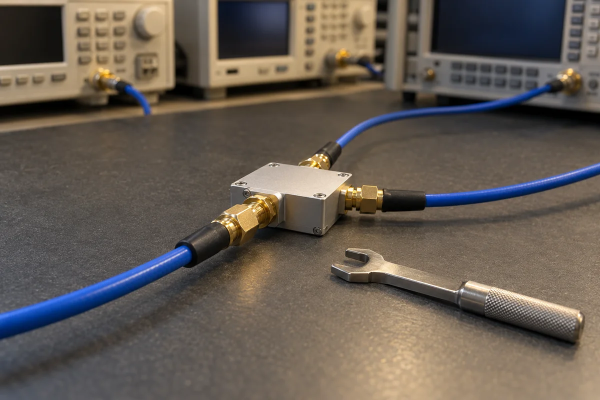
1. Choose the boundary. For total receiver rejection, inject ahead of the preselector. For mixer/combiner rejection alone, inject at that assembly’s RF input. Record the input plane and correct cable/path loss at each frequency.
2. Fix the receiver state. Record LO frequency and drive, gain settings, calibration state, output selection and terminations. Hold gain constant using the device’s test procedure so automatic gain control cannot change between tone measurements.
3. Apply the wanted tone. Measure its IF output power using an input level within the linear range. Keep the IF measurement bandwidth fixed.
4. Replace it with the image tone. Use the calculated image frequency and the same calibrated input level where practical. Measure the response at the same IF output.
5. Normalize and compare. Calculate rejection, check it against the allocated requirement including allowance, and repeat across the operating/image bands and relevant conditions.

With output readings O_D and O_I, and calibrated applied inputs I_D and I_I, all in dBm:

R_measured = (O_D − O_I) − (I_D − I_I), in dB.

The image response must remain distinguishable from the measurement floor. If it falls below that floor, report the rejection as a lower bound based on the measurement limit. Increasing the image input can improve visibility, provided the receiver remains linear and the input-power difference is included in the calculation. Keep this rejection measurement separate from the strong-blocker overload check.

LO, IF and image-rejection checklist

Carry the frequency plan and rejection budget into the same measurement record. The following checklist ties each input to a calculation or acceptance decision.

Record	Calculation or check
Wanted RF center and band edges; IF	Use consistent frequency units; confirm the nonzero-IF, positive-image model applies.
Injection side and LO setting	Calculate high-side and low-side plans; check LO tuning, drive and spectral orientation.
Image center and edges	Calculate 2f_LO − f_RF; reverse the mapped band endpoints at fixed LO.
Image blocker and desired input powers	Establish P_I − P_D at one stated input plane.
Required output margin and allowance	Set the total rejection requirement from P_I − P_D + M, then add allowance.
Filter loss at wanted and image bands	Record L_D, L_I and their difference A_pre over the required conditions.
Mixer and combining configuration	Record RF/LO/IF, selected output, hybrid or complex processing, terminations and calibration state.
Available mixer rejection	Compare its minimum over the required conditions with the residual budget.
Blocker headroom and noise	Check stage overload separately; include image noise generated after each filter.
Wanted/image response readings	Record calibrated input and IF output powers, bandwidth, temperature and measurement floor.
Acceptance	Pass the allocated rejection only when the normalized result meets the requirement and allowance; flag floor-limited results as bounds.

Technical references

• MITEQ, Image Rejection Mixers/QIFMs, printed catalog pages 254–256: Q1 for image frequency and LO selection; Q3 for equal-contribution noise folding; Q5 for combining; Q9 for LNA/filter placement.
• Analog Devices, Michael Dalton, AN-1258: Image Rejection Calibration on the ADF7021, ADF7021-N, and ADF7021-V: “Image Frequency Mechanism,” “Image Calibration Overview” and “Internal Tone Setup.”
• Mini-Circuits, IQ Mixers: Image Reject Down-Conversion & Single Sideband Up-Conversion: “Mixer Basics,” “Image Reject Mixers” and “Effect of Amplitude and Phase Unbalance on Image Rejection.”